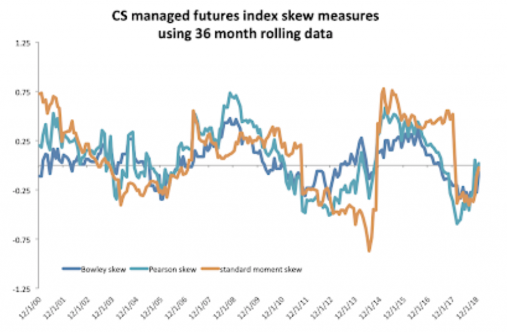
I was having a discussion about the merits of managed futures relative to other hedge fund styles. Managed futures funds will often have positive skew versus other hedge fund styles. The measurement of skew is tricky and is not present with all managers but for trend-followers who allow profits to accrue, it is more likely. The argument for positive skew is embedded in the behavior of the managers.
A trend-following CTA will structure their trades to create positive skew by holding onto winners and sell losers. More precisely, a manager who uses stop losses to reduce downside exposure and will follow trends for upside returns creates pay-offs which generate more upside potential. The profile shows many small loses with the opportunity for a few very strong gains.
The return pay-off will be like a synthetic option. If these synthetic options are created for both up and down markets, the result will be a profile like option straddles which are effectively employed to describe CTA performance.
Still, skew is not intuitive when described through the standard moment formula. Skew is referred to as the third moment of the distribution which is defined as the cubed scaled deviations from the mean or more precisely [(x – mean)/stdev]^3. Notice that it is easy to calculate and Excel will provide a normalized measure of skew. The skew can be tested for significance, but there are some simple rules of thumb. A skew above 1 is positive or below -1 negative. The range between plus and minus .5 is considered normal and the ranges between .5 and 1 or -.5 and -1 is considered mildly skewed.
If you say that a managers has positive skew of x, it does not tell the investor much about what excess returns they will actually be receiving other than the right tail of the distribution is pulled positive relative to a normal distribution. Volatility or fat tails may dominate any skew. A positively skewed distribution will actually be left leaning versus a normal distribution. The distribution is contorted away from symmetry around the mean. A positive (negative) skew will have a mean greater (less) than the median or mode.
There are different methods of looking at skew that may be more intuitive and provide a more useful means of thinking about skew. There are two Pearson measure of skew and the Bowley’s (Galton) quartile skewness measure. The Pearson measure is the difference between the mean and mode divided by the standard deviation. The Pearson second measure of skew measures three times the difference between the mean and median divided by the standard deviation. If the mean is higher than the median there is positive skew. This has a nice intuitive feel because it says that the average return is higher than the middle value of a return series. The Bowley measure looks at the difference in quartiles (q3+q1-2q2)/(q3-q1) which again has a simple intuitive appeal. If the third quartile is much further away from the median than the first quartile, the distribution has positive skew.
The skew will change through time based on sampling. Enclosed is a simple example of 36 month rolling average skew for the CS managed futures index. Notice that skew changes and the skew measures generate slightly different results. The moment skew which cubes deviations will have big changes when there are outliers. The Bowley skew based on quartile will not be as affected by outliers. The Pearson second skew coefficient will be sensitive to the difference between mean and median.

These differences are partially due to sampling and the mixture of samples. The skew will differ based on market conditions. The managed futures skew moved to strongly positive during the out-sized 2014 return period. Looking at the different measures of skew, the classic moment measure used in excel can generate big jumps when there is a large outlier. This is less likely to happen with the Pearson and Bowley measures.
